

Making polling averages react to campaign events
A dispatch from the Methods Desk


Polling averages have a hard job. On most days of a campaign, public opinion on a topic does not move meaningfully or predictably in either direction, and it especially does not move quickly. The lone exception is presidential approval, which in recent decades typically degrades little by little every day.
In the context of horse race polls, campaigns are stable, polls are noisy, and your average should really be quite steady. A trend line that twitches at every new survey is committing two errors: first, it’s reacting to noise in the data, a statistical error; and second, it’s really not adding anything journalistically anymore: readers can already see what the polls say, so an average should be able to tell them something more than whatever the latest survey showed.
Every once in a while, however, something actually happens that causes opinions to change. Campaign events like a candidate dropping out, a new scandal breaking, or a bad (or good!) debate performance can and do shape competitive races. A polling average that doesn’t move accordingly is missing something.
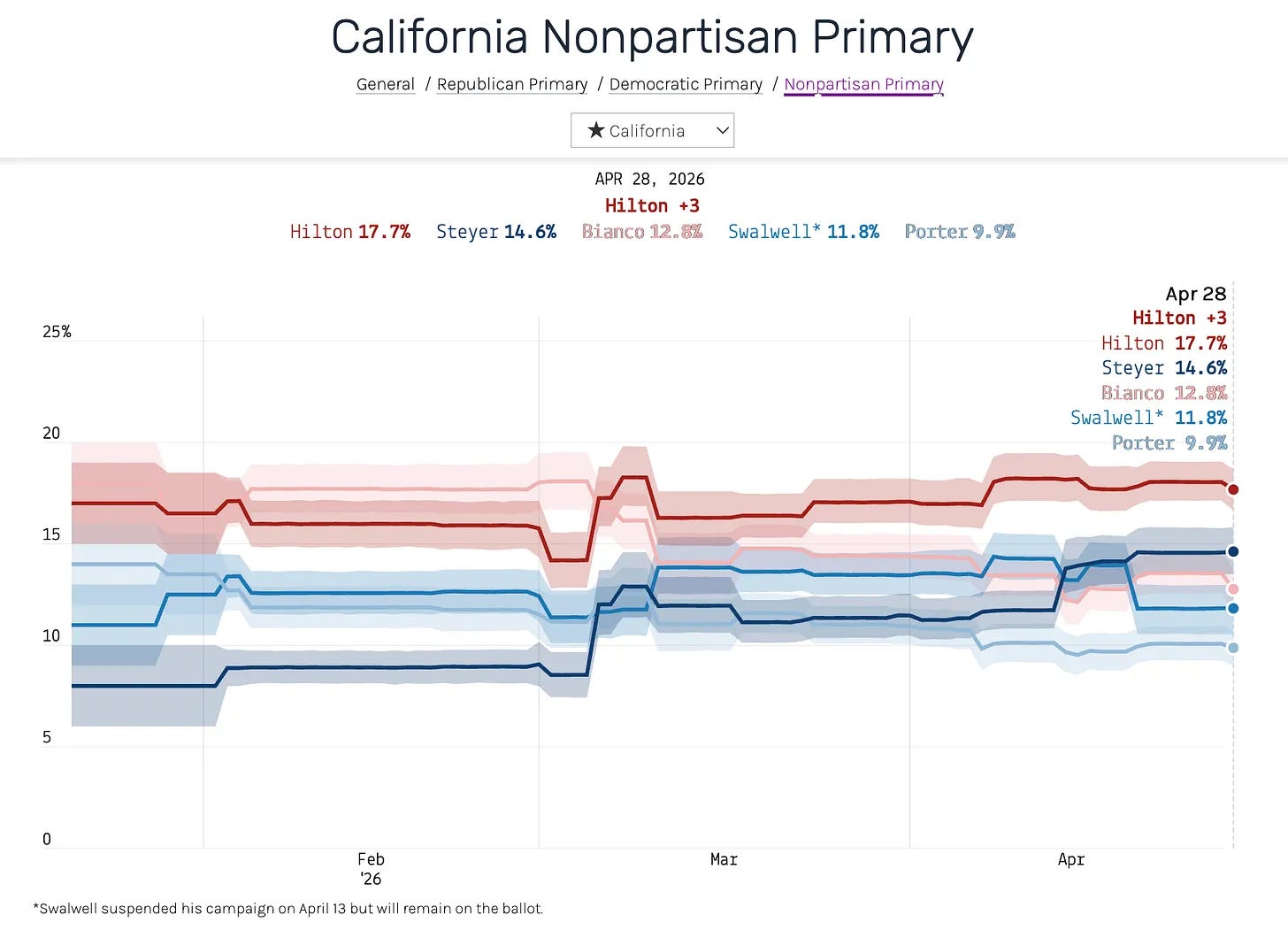
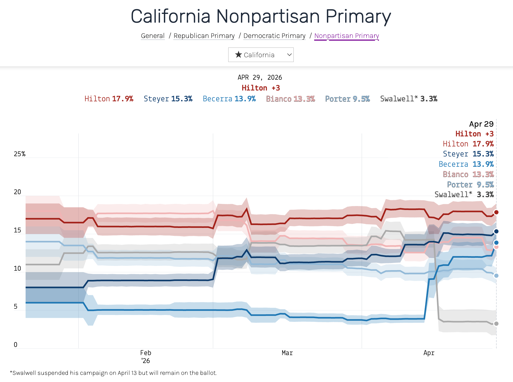
I’ve been thinking about this recently in the context of our average of polls for the upcoming California gubernatorial primary. Our polling average, as it appeared on April 28, 2026, appears below:

This is a reasonable average for a primary campaign that doesn’t have any major events going on. But that’s not what’s happening here. Former U.S. House Rep. Eric Swalwell suspended his campaign on April 13, following allegations of sexual misconduct from multiple women. More than two weeks later, our model still has him at 11.8% — within a point of where he’d been all spring (because Swalwell is still on the ballot, we have kept him on our average).
Yet support for Swalwell has actually plunged. Surveys taken after he suspended his campaign show him in the low single digits.
This model error is an interesting problem, from a statistics perspective, and worth walking readers through, because the same thing happens in every primary cycle and we want to use a polling average that can react to surprises when they happen. The fix we have come up with is also pretty satisfying, we think.
Why the model gets stuck
First, why is the average so stable in the first place?
The polling averages at 50+1 are powered by a statistical model detailed in full here. Each candidate has an underlying level of “true support” that evolves day to day as a random walk over time. Statistically, this is formulated as:
average[today] = average[yesterday] + step[today]Where step[today] is a number that is drawn from a statistical distribution called a Laplace distribution that looks like this:
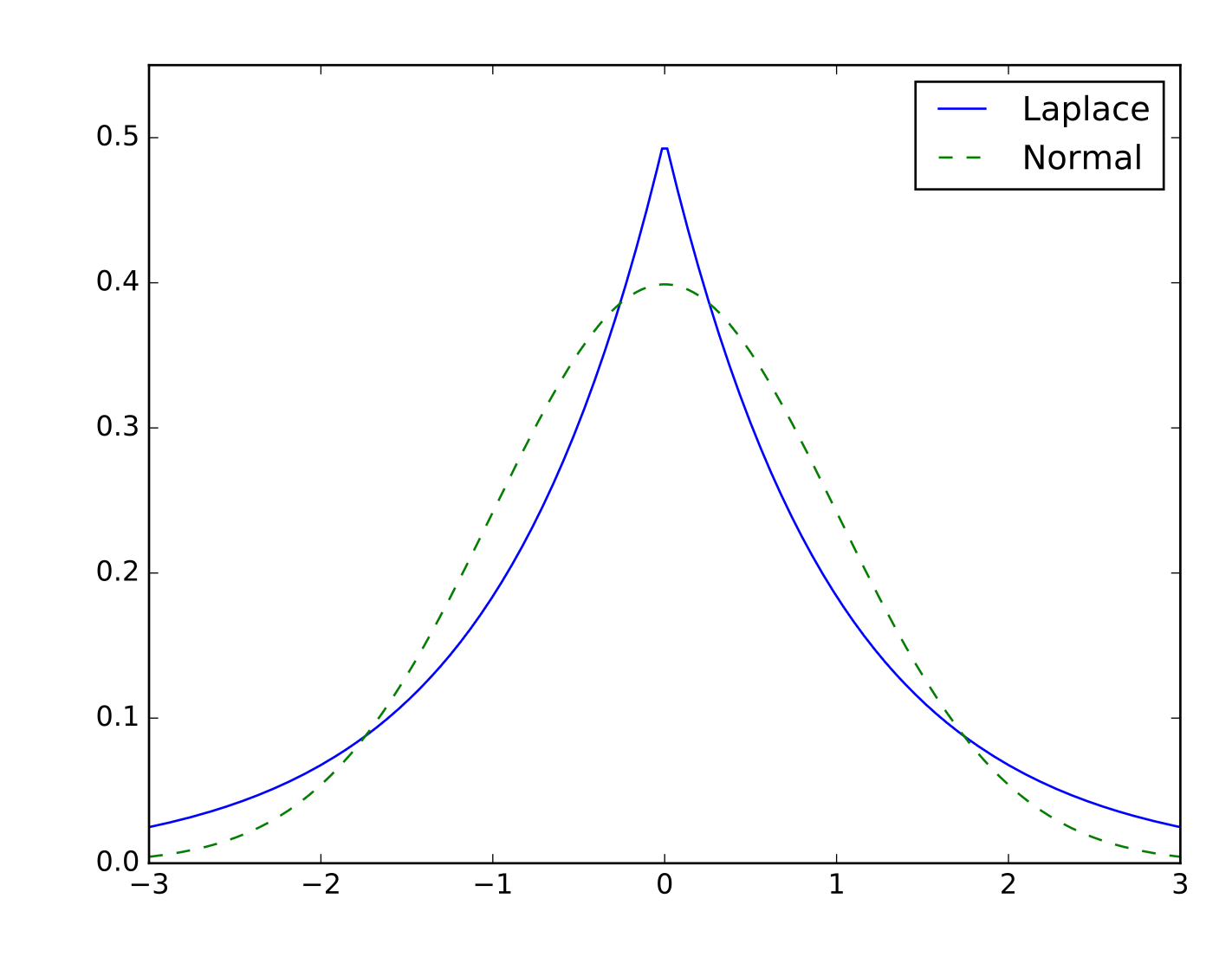
This distribution allows for both a higher occurrence of extreme values and a higher concentration of zeroes than the normal or other fat-tailed distribution. We use the Laplace distribution because, as theorized above, we don’t want the polling average to move around too much from day to day — but on days that campaign events happen, we want the average to be able to make big jumps.
We call these jumps ‘steps’ in the statistical parlance. Every day, the polling average is allowed to move up or down by a certain amount, which we call average_change.
Formally,
step[today] ~ laplace(0, average_change)The parameter average_change controls how much the trend is allowed to move per day. A small value gives a smooth line; a larger one gives a jumpier line. We estimate average_change as a parameter in our statistical model, meaning it’s allowed to have a high value in races where opinions are volatile (hello, CA-Gov!) and a small value in other races. Usually the value is about 0.3 percentage points per day — small enough that the model expects gentle drift in opinion, with very occasional jumps.
Because we are Bayesians here at 50+1, we do not fit this model completely from scratch. Each day’s value for average is softly anchored to a simple exponentially-weighted moving average (EWMA) of the non-partisan polls in a race. This anchor serves two purposes: first, it allows us to incorporate other averaging techniques in our average (we are not perfect); and second, it dramatically speeds up the runtime of the computer program that powers our averages.
So this means that support for a candidate on a given day depends on three variables: the previous day’s level of support, the soft anchor from the EWMA, and today’s new poll observations. In normal times this works beautifully: you get a smooth curve of opinion with medium-sized jumps when a normal campaign event like a debate or a gaffe happens. The model’s estimates are exactly as smooth as you want.
But as any modeler knows, the real world can be quite messy. When a a non-normal event happens that changes the dynamics of a race overnight — we call these “shocks” — two of the variables above become statistical liabilities:
The random-walk prior says huge day-to-day moves are unlikely. Because the model’s
average_changeparameter is fit to account for big campaign shocks in the tails of the distribution, shocks that are even more extreme get washed out as noise.The EWMA anchor still includes old, pre-shock polls, pulling the trend toward the old level. Even if the random walk loosened up, the anchor would yank the trend back.
The normal model that is walking around the world, whistling as it processes a steady stream of data that fits its idea of what a “normal” event is, is caught off guard by the shock.
How do we fix this?
Fix 1: Tell the model when a big campaign event happened, and let the average jump around after
Our first move is to tell the model when shocks occur, and to let it move the average dramatically to account for new polling if it decides to. After a campaign shock, the model inflates the average_change variable so the trend can jump around.
Concretely, we convert the single variable average_change to a vector of individual daily change values (called daily_change) that varies over time, instead of being a single fixed value. Before a shock, daily_change is equal to the value of average_change. But on the day a shock happens, daily_change jumps up by some multiplier value (the default ×10) to let the model move the polling average more. Each subsequent day, the value of daily_change decays exponentially back down to its baseline, returning to the normal level in about 14 days.
By making this change, we allow both a candidate’s average level of support and our certainty about it to change over time. We’ve encoded our prior knowledge from observing campaign events that a big jump is plausible right now.
To be clear, we have not told model what direction to jump, only that a big jump is now possible. The data still drives what direction the model moves, we’ve just temporarily removed the penalty on big jumps that would otherwise get suppressed by even a fat-tailed distribution. (Readers who work in finance will clock this as similar to a stochastic volatility model).
Fix 2: Re-anchor the average to an updated, post-shock prior
But loosening the random walk alone isn’t enough. The model still has its prior trend — the EWMA run on all the polls — that is averaging together a bunch of pre-shock data. This pulls the final trend toward the old one, even with the wider variance on the daily steps.
So on and after a shock day, we calculate an additional new EWMA that only consists of the data taken after the campaign shock. Then we average this new, post-shock EWMA with the usual, full-period EWMA, giving 80% of the weight in that average to the fast-moving EWMA and 20% on the older one.
This 80/20 blend makes sure the post-EWMA average doesn’t get pulled around by noise in polls. If we anchored the new average just to post-shock polls, we would let one or two early polls dictate the new level of the model, which adds a lot of noise to the average. The 20% weight on the full-period EWMA stabilizes the anchor when post-shock data is thin, and its influence shrinks naturally as more post-shock polls accumulate (and as we move away from the shock).
Methodologically this is equivalent to telling the model that the unobserved process changed regimes at the shock date, so older polls are partially informative about the new regime but not fully.
A newer, faster-moving average — when it’s warranted
To refresh your memory, here is what the old CA gubernatorial primary average looked like:
And here’s the same race, with the same polls, using the new model:
The Swalwell line now does what we would expect it to a priori and takes a sharp drop in mid-April, settling at 3.2% by April 29 — about where the post-scandal polls have him. We also added a new line (in medium-blue color) for Xavier Becerra, the former secretary of health and human services who has gained a lot since Swalwell dropped out. (Our rule of thumb is to include candidates in our polling averages if they are routinely polling above 5%. That wasn’t true of Becerra before Swalwell suspended his campaign, but it is true now.)
Tunable parameters
To recap for anyone running a similar version of our average at home, we have introduced three new variables that the model can tune appropriately:
shock_multiplier(default 10): The peak multiplicative factor on the value ofaverage_changeon the day a big shock occurred. Higher means bigger jumps in the average.shock_decay(default ln(10)/14 ≈ 0.165 per day, or a return to normal variance 2 weeks after the campaign shock): Higher means a shorter window of elevated variance.post_shock_weight(default 0.8): weight on the post-shock EMA in the blended anchor. Higher is more responsive, less stable.
Both shock_multiplier and shock_decay are estimated as parameters in our Bayesian model, run in the programming language Stan, with the user-supplied values acting as priors on these values. So the defaults are starting points, not hard settings — the data can pull them in either direction. The post_shock_weight is specified in an ad-hoc way, and we can probably improve the average by testing different values on historical primaries.
Closing thoughts
Coding a polling averages requires making a tradeoff between stability and reactivity, and there is no single model that works perfectly for every race. A model tuned to react quickly to shocks will jitter through ordinary noise; a model tuned for stability will sit through real events.
The best way to resolve this tension is to make the model conditional on whether something has happened — quiet most days, willing to move on the days that count. We have resisted doing this in the past because it means assembling a dataset of campaign shocks over every race we are monitoring, and all the races in our historical polling data. But we think the extra effort is worth the gains in accuracy.
We will now be using this accommodating average for all primary campaigns, and are testing it on general election averages too. We are not immediately planning to move the presidential approval or generic ballot averages over to the model with hard, user-specified shocks, because in our research these polls tend to react more predictably to the historical range of real-world events. But if something does happen, we now have a framework for enabling the same degree of reactivity in those contexts, too.
Paid subscribers to 50+1 get access to premium analysis, plus sortable tables and complete data access on our polling website. If you want to follow the 2026 cycle with the best data at your fingertips, become a paid subscriber.
Thanks, I'd quit looking at your CA primary tracker for that reason.
If I read this right, you're manually injecting an impact to the model, though I understand you're not impacting _data_ that is introduced into the model.
It also strikes me that in primaries there is less polling and more "events", like candidates dropping out.
I see that you specify *Swalwell at the bottom in addition by his name on the right. It would be good to make it your standard practice to identify all such times that you make this manual instruction to the model.
Interesting explanation of how sudden changes are handled in polls. What happens when there are much fewer candidates in a race. As an example 3 candidates and all polling at 20 percent or higher and one of these candidates essentially flames out like Swalwell did? Would your fixes show the impacts of that event sooner?